Run in Google Colab

Autoencoders in SciKeras

Autencoders are an approach to use nearual networks to distill data into it’s most important features, thereby compressing the data. We will be following the Keras tutorial on the topic, which goes much more in depth and breadth than we will here. You are highly encouraged to check out that tutorial if you want to learn about autoencoders in the general sense.

Table of contents

• 1. Setup

• 2. Data

• 3. Define Keras Model

• 4. Training

• 5. Explore Results

1. Setup

try:
    import scikeras
except ImportError:
    !python -m pip install scikeras

Silence TensorFlow logging to keep output succinct.

import warnings
from tensorflow import get_logger
get_logger().setLevel('ERROR')
warnings.filterwarnings("ignore", message="Setting the random state for TF")

import numpy as np
from scikeras.wrappers import KerasClassifier, KerasRegressor
from tensorflow import keras

2. Data

We load the dataset from the Keras tutorial. The dataset consists of images of cats and dogs.

from tensorflow.keras.datasets import mnist
import numpy as np


(x_train, _), (x_test, _) = mnist.load_data()
x_train = x_train.astype('float32') / 255.
x_test = x_test.astype('float32') / 255.
x_train = x_train.reshape((len(x_train), np.prod(x_train.shape[1:])))
x_test = x_test.reshape((len(x_test), np.prod(x_test.shape[1:])))
print(x_train.shape)
print(x_test.shape)

Downloading data from https://storage.googleapis.com/tensorflow/tf-keras-datasets/mnist.npz
11493376/11490434 [==============================] - 0s 0us/step
(60000, 784)
(10000, 784)

3. Define Keras Model

We will be defining a very simple autencoder. We define three model building methods:

1. One to build a full end-to-end autoencoder.

2. One to create a model that includes only the encoder portion.

3. One that creates a model that includes only the decoder portion.

The only variable we give our model is the encoding dimensions, which will be a hyperparemter of our final transformer.

from tensorflow import keras


def get_fit_model(encoding_dim: int) -> keras.Model:
    """Get an autoencoder.

    This autoencoder compresses a 28x28 image (784 pixels) down to a feature of length
    `encoding_dim`, and tries to reconstruct the input image from that vector.
    """
    input_img = keras.Input(shape=(784,), name="input")
    encoded = keras.layers.Dense(encoding_dim, activation='relu', name="encoded")(input_img)
    decoded = keras.layers.Dense(784, activation='sigmoid', name="output")(encoded)
    autoencoder_model = keras.Model(input_img, decoded)
    return autoencoder_model

def get_tf_model(fit_model: keras.Model) -> keras.Model:
    """Get an encoder model.

    We do this by extracting the encoding layer from the fitted autoencoder model.
    """
    return keras.Model(fit_model.get_layer("input").input, fit_model.get_layer("encoded").output)

def get_inverse_tf_model(fit_model: keras.Model, encoding_dim: int) -> keras.Model:
    """Get an deencoder model.

    We do this by extracting the deencoding layer from the fitted autoencoder model
    and adding a new Keras input layer.
    """
    encoded_input = keras.Input(shape=(encoding_dim,))
    output = fit_model.get_layer("output")(encoded_input)
    return keras.Model(encoded_input, output)

Next we create a class that that will enable the transform and fit_transform methods, as well as integrating all three of our models into a single estimator.

from sklearn.base import TransformerMixin, clone
from scikeras.wrappers import BaseWrapper


class KerasTransformer(BaseWrapper, TransformerMixin):
    """A class that enables transform and fit_transform.
    """

    def __init__(self, *args, tf_est: BaseWrapper = None, inv_tf_est: BaseWrapper = None, **kwargs) -> None:
        super().__init__(*args, **kwargs)
        self.tf_est = tf_est
        self.inv_tf_est = inv_tf_est


    def fit(self, X, sample_weight=None):
        super().fit(X=X, y=X, sample_weight=sample_weight)
        self.tf_est_ = clone(self.tf_est)
        self.inv_tf_est_ = clone(self.inv_tf_est)
        self.tf_est_.set_params(fit_model=self.model_)
        self.inv_tf_est_.set_params(fit_model=self.model_, encoding_dim=self.encoding_dim)
        X = self.feature_encoder_.transform(X)
        self.tf_est_.initialize(X=X)
        X_tf = self.tf_est_.predict(X=X)
        self.inv_tf_est_.initialize(X_tf)
        return self

    def transform(self, X):
        X = self.feature_encoder_.transform(X)
        X_tf = self.tf_est_.predict(X)
        return X_tf

    def inverse_transform(self, X_tf):
        X = self.inv_tf_est_.predict(X_tf)
        X = self.feature_encoder_.inverse_transform(X)
        return X

Next, we wrap the Keras Model with Scikeras. Note that for our encoder/decoder estimators, we do not need to provide a loss function since no training will be done. We do however need to have the fit_model and encoding_dim so that these will be settable by BaseWrapper.set_params.

tf_est = BaseWrapper(model=get_tf_model, fit_model=None, verbose=0)
inv_tf_est = BaseWrapper(model=get_inverse_tf_model, fit_model=None, encoding_dim=None, verbose=0)
autoencoder = KerasTransformer(model=get_fit_model, tf_est=tf_est, inv_tf_est=inv_tf_est, loss="binary_crossentropy", encoding_dim=32, epochs=5)

4. Training

To train the model, we pass the input images as both the features and the target. This will train the layers to compress the data as accurately as possible between the encoder and decoder. Note that we only pass the X parameter, since we defined the mapping y=X in KerasTransformer.fit above.

_ = autoencoder.fit(X=x_train)

Epoch 1/5
1875/1875 [==============================] - 4s 2ms/step - loss: 0.2033
Epoch 2/5
1875/1875 [==============================] - 4s 2ms/step - loss: 0.1049
Epoch 3/5
1875/1875 [==============================] - 4s 2ms/step - loss: 0.0972
Epoch 4/5
1875/1875 [==============================] - 3s 2ms/step - loss: 0.0959
Epoch 5/5
1875/1875 [==============================] - 3s 2ms/step - loss: 0.0949

Next, we round trip the test dataset and explore the performance of the autoencoder.

roundtrip_imgs = autoencoder.inverse_transform(autoencoder.transform(x_test))

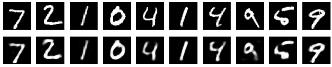
5. Explore Results

Let’s compare our inputs to lossy decoded outputs:

import matplotlib.pyplot as plt


n = 10  # How many digits we will display
plt.figure(figsize=(20, 4))
for i in range(n):
    # Display original
    ax = plt.subplot(2, n, i + 1)
    plt.imshow(x_test[i].reshape(28, 28))
    plt.gray()
    ax.get_xaxis().set_visible(False)
    ax.get_yaxis().set_visible(False)

    # Display reconstruction
    ax = plt.subplot(2, n, i + 1 + n)
    plt.imshow(roundtrip_imgs[i].reshape(28, 28))
    plt.gray()
    ax.get_xaxis().set_visible(False)
    ax.get_yaxis().set_visible(False)
plt.show()

What about the compression? Let’s check the sizes of the arrays.

encoded_imgs = autoencoder.transform(x_test)
print(f"x_test.shape[1]: {x_test.shape[1]}")
print(f"encoded_imgs.shape[1]: {encoded_imgs.shape[1]}")
cr = round((encoded_imgs.nbytes/x_test.nbytes), 2)
print(f"Compression ratio: 1/{1/cr:.0f}")

x_test.shape[1]: 784
encoded_imgs.shape[1]: 32
Compression ratio: 1/25